Easy Vitessce Documentation#
Easy Vitessce is a Python package for turning Scanpy and SpatialData plots into interactive Vitessce visualizations with minimal code changes.
Installation#
Requires Python 3.10 or greater.
pip install easy_vitessce
How to Use and Examples#
The package can be imported with
import easy_vitessce as ev
By default, interactive plots are enabled via running this import statement.
Deactivating/Reactivating Interactive Plots#
Run ev.disable_plots to deactivate Vitessce plots.
Run ev.enable_plots to re-activate Vitessce plots.
ev.disable_plots(["embedding", "violin", "spatialdata-plot"])

ev.enable_plots(["spatialdata-plot", "violin"])
Spatial Plot (SpatialData-Plot version)#
Note: This example uses SpatialData’s mouse brain MERFISH dataset.
sdata = sd.read_zarr(spatialdata_filepath)
sdata.pl.render_images(element="rasterized").pl.render_shapes(element="cells", color="Acta2").pl.show()
spatialdata_filepath should lead to a .zarr file containing spatial data with an Images folder. The file structure of the example above is as follows. Since it does not have a Labels folder, calling pl.render_labels() will not display any data.
SpatialData object, with associated Zarr store:
├── Images
│     └── 'rasterized': DataArray[cyx] (1, 522, 575)
├── Points
│     └── 'single_molecule': DataFrame with shape: (<Delayed>, 3) (2D points)
├── Shapes
│     ├── 'anatomical': GeoDataFrame shape: (6, 1) (2D shapes)
│     └── 'cells': GeoDataFrame shape: (2389, 2) (2D shapes)
└── Tables
      └── 'table': AnnData (2389, 268)
![]()
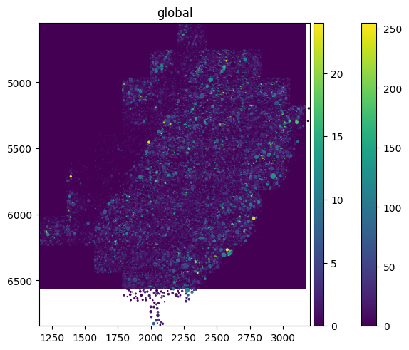
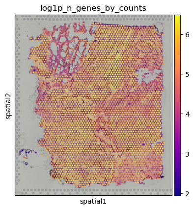
Spatial Plot (Scanpy version)#
Easy Vitessce’s spatial function also displays a spatial plot, but with Scanpy’s syntax. This example uses Scanpy’s Visium dataset.
adata = sc.datasets.visium_sge(sample_id="Targeted_Visium_Human_Glioblastoma_Pan_Cancer", include_hires_tiff=True)

sc.pl.spatial(adata, color = "log1p_n_genes_by_counts")
![]()
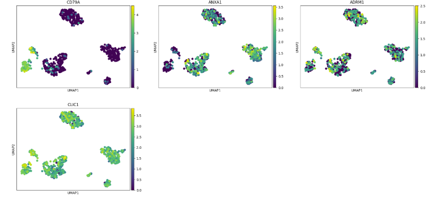
Scatterplots#
Easy Vitessce’s embedding function displays UMAP, PCA, and t-SNE scatterplots.
The functions umap, pca, and tsne can also be used for convenience.
adata = sc.datasets.pbmc68k_reduced()

sc.pl.embedding(adata, basis="X_umap", color="CD79A")
sc.pl.embedding(adata, basis="X_pca", color=["CD79A", "CD53"])
sc.pl.embedding(adata, basis="X_tsne", color=["bulk_labels", "louvain", "phase"])

sc.pl.umap(adata, color="CD79A")
sc.pl.pca(adata, color="CD79A")
sc.pl.tsne(adata, color="CD79A")
![]()
Dotplot#
Note: To select/deselect multiple genes, hold SHIFT while clicking on genes in the Gene List.
adata = sc.datasets.pbmc68k_reduced()

sc.pl.dotplot(adata, var_names=["C1QA", "PSAP", "CD79A", "CD79B", "CST3", "LYZ"], groupby="bulk_labels")

![]()
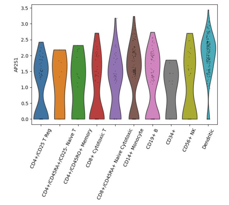
Violin Plot#
adata = sc.datasets.pbmc68k_reduced()

sc.pl.violin(adata, keys="AP2S1", groupby="bulk_labels")
![]()
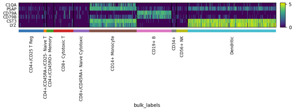
Heatmap#
adata = sc.datasets.pbmc68k_reduced()

sc.pl.heatmap(adata, groupby="bulk_labels", var_names=['C1QA', 'PSAP', 'CD79A', 'CD79B', 'CST3', 'LYZ'])
![]()
Citation#
To cite EasyVitessce in your work, please use:
S Luo, MS Keller, T Kakar, L Choy, N Gehlenborg. “EasyVitessce: auto-magically adding interactivity to Scverse single-cell and spatial biology plots”, arXiv (2025). doi:10.48550/arXiv.2510.19532